Advanced Google Cloud Load Balancing & Cloud Armor Analytics with Custom Dashboards
Gaining deeper insights into your Google Cloud load balancer traffic and Cloud Armor policies is essential for improving performance and security. While Google Cloud provides some built-in dashboards, they often lack the depth required for detailed traffic analysis. Learn how to build advanced analytics dashboards with BigQuery, Grafana and Terraform, enabling functionalities found in solutions like Cloudflare.
What Already Exists
Google Cloud provides the following built-in dashboards:
- External HTTP(S) Load Balancers Dashboard: Available under Monitoring > Dashboards > External HTTP(S) Load Balancers. This dashboard provides insights into error rates and latency percentiles per forwarding rule.
- Network Security Policies Dashboard: Found under Monitoring > Dashboards > Network Security Policies, this dashboard gives an overview of request rates for Cloud Armor policies, including how many requests were allowed or blocked.
- Cloud Armor Insights: Additional Cloud Armor policy information can be found under Security > Findings > Quick Filters > Cloud Armor.
What We Want
The built-in dashboards are useful for basic monitoring, but they lack flexibility and detailed analytics. We want dashboards that offer: Group-by, filter, and Top N analysis on:
- Source IPs
- Hosts
- Paths
- Status codes
- Query parameters
- HTTP request methods
- Source countries
- Action taken (blocked, allowed, throttled)
- etc.
This level of granularity is provided by, for example, Cloudflare’s Security Analytics.
Building Advanced Load Balancer Analytics in Google Cloud
Enable Logging for Backend Services
Dashboards rely on request logs generated by backend services. Since logging is disabled by default, you’ll need to enable it for the services you wish to analyze. See the documentation for instructions: Enabling Logging. Similarly, you can also enable backend service logging for GKE’s Gateway API:
apiVersion: networking.gke.io/v1
kind: GCPBackendPolicy
metadata:
  name: "example"
spec:
  default:
    logging:
      enabled: true
      sampleRate: 100000 # out of 1,000,000
The sample rate determines the percentage of requests that are logged. A higher rate provides more data but increases costs. Start with, for example, 10% sample rate and adjusting it based on your analysis needs and budget.
Route Logs to a BigQuery Dataset
For efficient analysis of potentially billions of generated logs, route them to BigQuery. Begin by creating a BigQuery dataset: Create Datasets, or with Terraform:
resource "google_bigquery_dataset" "this" {
  dataset_id  = "lb_logs"
  description = "Dataset containing logs for any requests made to the LB in the past 30 days."
  location    = local.location

  default_partition_expiration_ms = 31 * 24 * 60 * 60 * 1000 # 31 days

  storage_billing_model = "PHYSICAL"

  lifecycle {
    prevent_destroy = true
  }
}
To send your logs to BigQuery, you’ll need to create a log sink. Navigate to Log Router in Cloud Logging and create a new sink: Route logs to supported destinations. Set the destination to your lb_logs BigQuery dataset. It's crucial to filter the logs to include only the relevant ones. With Terraform:
resource "google_logging_project_sink" "this" {
  name = "lb_logs"

  destination = "bigquery.googleapis.com/projects/${var.project}/datasets/${google_bigquery_dataset.this.dataset_id}"

  unique_writer_identity = true

  bigquery_options {
    use_partitioned_tables = true
  }

  filter = join("", [
    # only LB logs
    "resource.type=\"http_load_balancer\" AND ",
    # optionally, only from specific LB, for example in this case GKE Kubernetes Gateway API
    "resource.labels.target_proxy_name=\"${
      reverse(
        split("/",
          data.kubernetes_resource.gateway_external_direct.object.metadata.annotations["networking.gke.io/target-https-proxies"]
        )
      )[0]
    }\" AND ",
    # optionally, include only traffic that is protected with cloud armor (vast majority anyway)
    "jsonPayload.enforcedSecurityPolicy.name:*"
    ]
  )
}

resource "google_bigquery_dataset_iam_member" "sink_writer" {
  dataset_id = google_bigquery_dataset.this.dataset_id
  role       = "roles/bigquery.dataEditor"
  member     = google_logging_project_sink.this.writer_identity
}

data "kubernetes_resource" "gateway" {
  api_version = "gateway.networking.k8s.io/v1"
  kind        = "Gateway"

  metadata {
    name      = "gateway"
    namespace = "gateway"
  }
}
Optionally, you can add an exclusion filter to the _Default log sink. This prevents load balancer logs from being stored in both the default logging bucket and your lb_logs BigQuery dataset, avoiding unnecessary storage costs.
Materialized View
After enabling backend service logging and creating a log sink, a requests table will automatically appear (on first generated log) in your lb_logs BigQuery dataset. To optimize query costs and ensure the data is in the correct format for our dashboards, we recommend creating a materialized view: Create materialized views. This view should aggregate data at 1-minute or 5-minute intervals, and you should also partition the table by day and add clustering for even greater cost savings. With Terraform:
resource "google_bigquery_table" "time_bucket_agg" {
  project     = var.project
  dataset_id  = google_bigquery_dataset.this.dataset_id
  table_id    = "time_bucket_agg"
  description = "Extracts the relevant LB traffic data and aggregates it into time buckets."

  materialized_view {
    query = <<EOT
SELECT
  TIMESTAMP_TRUNC(timestamp, DAY) AS date,
  DATETIME_BUCKET(timestamp, INTERVAL 5 MINUTE) AS time_bucket,
  jsonpayload_type_loadbalancerlogentry.enforcedsecuritypolicy.name AS waf_policy_name,
  jsonpayload_type_loadbalancerlogentry.enforcedsecuritypolicy.outcome AS waf_outcome,
  jsonpayload_type_loadbalancerlogentry.enforcedsecuritypolicy.configuredaction AS waf_configured_action,
  NET.HOST(httpRequest.requesturl) AS host,
  httpRequest.remoteip AS source_ip,
  REGEXP_EXTRACT(httpRequest.requesturl, r'https?://[^/]+(/[^?]*)') AS path,
  REGEXP_EXTRACT(httpRequest.requesturl, r'\?([^#]+)') AS query_params,
  COUNT(*) AS requests
FROM
  `${google_bigquery_dataset.this.dataset_id}.requests`
GROUP BY
  date,
  time_bucket,
  waf_policy_name,
  waf_outcome,
  waf_configured_action,
  host,
  source_ip,
  path,
  query_params
EOT
  }

  time_partitioning {
    type          = "DAY"
    field         = "date"
    expiration_ms = 31 * 24 * 60 * 60 * 1000 # 31 days
  }

  clustering = [
    "source_ip",
    "host",
    "path",
    "query_params"
  ]

  deletion_protection = true
}
Visualize with Grafana
With your data in BigQuery and the materialized view created, you can now build dashboards. This post focuses on Grafana, but the same ideas apply to Google Cloud dashboards.
Create BigQuery Data Source
Before you can visualize your BigQuery data in Grafana, you need to add a BigQuery data source. This involves two steps:
- Install the BigQuery plugin
- Create a Google Cloud service account with appropriate permissions and create the data source in Grafana. With Terraform:
resource "google_service_account" "bigquery" {
  project    = var.project
  account_id = "grafana-big-query"
}

resource "google_project_iam_member" "bigquery_data_viewer" {
  project = var.project
  role    = "roles/bigquery.dataViewer"

  member = "serviceAccount:${google_service_account.bigquery.email}"
}

resource "google_project_iam_member" "bigquery_job_user" {
  project = var.project
  role    = "roles/bigquery.jobUser"

  member = "serviceAccount:${google_service_account.bigquery.email}"
}

resource "google_service_account_key" "bigquery_key" {
  service_account_id = google_service_account.bigquery.name
}

resource "grafana_data_source" "bigquery" {
  type = "grafana-bigquery-datasource"
  name = "BigQuery"
  uid  = "bigquery"

  json_data_encoded = jsonencode({
    authenticationType = "jwt"
    clientEmail        = google_service_account.bigquery.email
    defaultProject     = var.project
    tokenUri           = "https://oauth2.googleapis.com/token"
    MaxBytesBilled     = 1024*1024 # determined by your use case
    processingLocation = "your-location"
  })

  secure_json_data_encoded = jsonencode({
    privateKey = jsondecode(base64decode(google_service_account_key.bigquery_key.private_key)).private_key
  })
}
Create Dashboard Variables
After verifying your BigQuery data source works, you can start building your dashboards. Define the following dashboard variables:
- interval:
5m,15m,30m,1h,6h,1d - group_by:
waf_outcome,waf_configured_action,waf_policy_name,host,source_ip, path,query_params - source_ip
- waf_outcome_filter:
DENY,ACCEPT - waf_configured_action_filter:
ALLOW,THROTTLE,DENY - waf_policy_name_filter
- host_filter
- path_filter
- query_params_filter
- sample_rate: (Your backend service’s sample rate, e.g., 0.1 for 10%)
Create Top 10s Panels
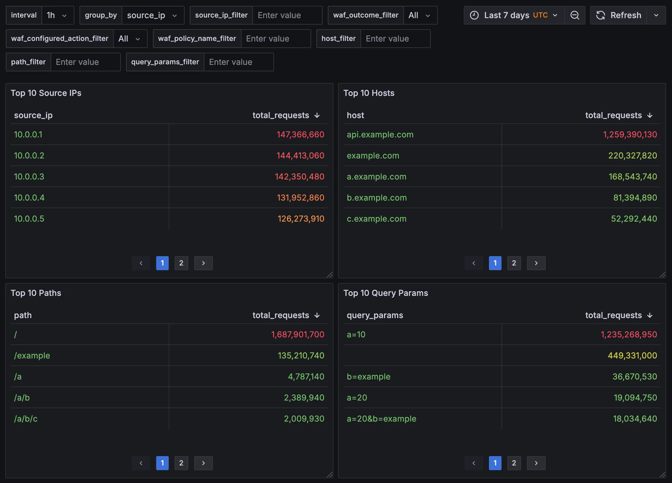
Creating Top 10 panels follows a similar pattern: consider the time range, apply filters, and group by the desired column. For example, here’s how to create a Top 10 Source IPs panel:
SELECT
    source_ip,
    SUM(requests) / ${sample_rate:raw} AS total_requests
  FROM
    `lb_logs.time_bucket_agg`
  WHERE
    date >= TIMESTAMP_TRUNC(TIMESTAMP_MILLIS(${__from}), DAY) AND date <= TIMESTAMP_TRUNC(TIMESTAMP_MILLIS(${__to}), DAY)
    AND $__timeFilter(time_bucket)
    AND ('${source_ip_filter:raw}' = '' OR source_ip = '${source_ip_filter:raw}')
    AND ('${waf_outcome_filter:raw}' = 'All' OR waf_outcome = '${waf_outcome_filter:raw}')
    AND ('${waf_configured_action_filter:raw}' = 'All' OR waf_configured_action = '${waf_configured_action_filter:raw}')
    AND ('${waf_policy_name_filter:raw}' = '' OR waf_policy_name = '${waf_policy_name_filter:raw}')
    AND ('${host_filter:raw}' = '' OR host = '${host_filter:raw}')
    AND ('${path_filter:raw}' = '' OR path = '${path_filter:raw}')
    AND ('${query_params_filter:raw}' = '' OR query_params = '${query_params_filter:raw}')
  GROUP BY
    source_ip
  ORDER BY total_requests DESC
  LIMIT 10
Before your query reaches BigQuery, Grafana substitutes its template variables (like ${grafana_variable}). Although all defined filters are included in the query string, BigQuery's query optimizer is smart enough to remove any unnecessary filters.
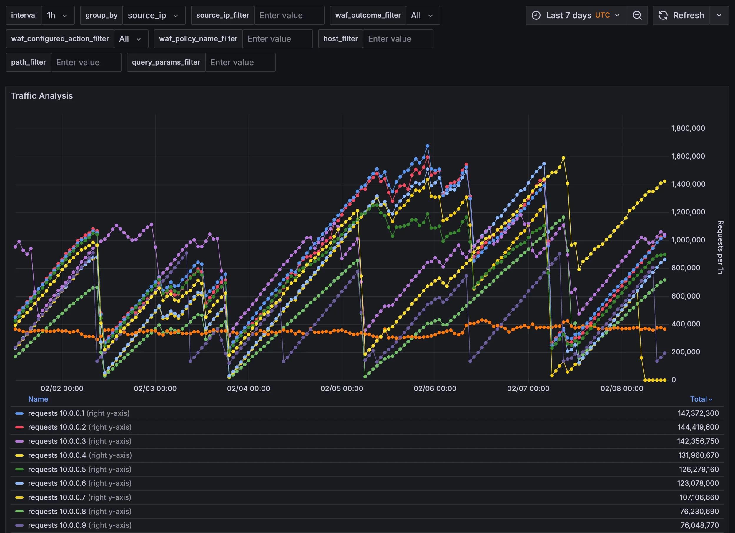
Create Traffic Analysis Panel
The Traffic Analysis panel is more complex because grouping by some dimensions like source_ip can produce thousands of lines to diagram. Therefore, it's essential to limit the results to the top 10.
-- When group_by is set to, for example, source_ip and there is no source_ip_filter
-- make sure that we don't potentially return enormous amounts of data, but only for top X IPs.
-- If this query is not actually used in the where statements of the main query,
-- it's optimized away
WITH top_10_x AS (
SELECT
    ${group_by:raw}
  FROM
    `lb_logs.time_bucket_agg`
  WHERE
    date >= TIMESTAMP_TRUNC(TIMESTAMP_MILLIS(${__from}), DAY) AND date <= TIMESTAMP_TRUNC(TIMESTAMP_MILLIS(${__to}), DAY)
    AND $__timeFilter(time_bucket)
    AND ('${waf_outcome_filter:raw}' = 'All' OR waf_outcome = '${waf_outcome_filter:raw}')
    AND ('${waf_configured_action_filter:raw}' = 'All' OR waf_configured_action = '${waf_configured_action_filter:raw}')
    AND ('${waf_policy_name_filter:raw}' = '' OR waf_policy_name = '${waf_policy_name_filter:raw}')
    AND ('${host_filter:raw}' = '' OR host = '${host_filter:raw}')
    AND ('${path_filter:raw}' = '' OR path = '${path_filter:raw}')
    AND ('${query_params_filter:raw}' = '' OR query_params = '${query_params_filter:raw}')
  GROUP BY
    ${group_by:raw}
  ORDER BY SUM(requests) DESC
  LIMIT 10
)

SELECT
  $__timeGroup(time_bucket, $interval) AS time_bucket_grafana,
  ${group_by:raw},
  SUM(requests) / ${sample_rate:raw} AS requests
FROM
  `lb_logs.time_bucket_agg`
WHERE
  date >= TIMESTAMP_TRUNC(TIMESTAMP_MILLIS(${__from}), DAY) AND date <= TIMESTAMP_TRUNC(TIMESTAMP_MILLIS(${__to}), DAY)
  AND $__timeFilter(time_bucket)
  -- source_ip conditions
  AND (
    ('${source_ip_filter:raw}' != '' AND source_ip = '${source_ip_filter:raw}') OR
    ('${source_ip_filter:raw}' = '' AND '${group_by:raw}' != 'source_ip') OR
    ('${source_ip_filter:raw}' = '' AND '${group_by:raw}' = 'source_ip' AND source_ip IN (SELECT source_ip FROM top_10_x))
  )
  -- host conditions
  AND (
    ('${host_filter:raw}' != '' AND host = '${host_filter:raw}') OR
    ('${host_filter:raw}' = '' AND '${group_by:raw}' != 'host') OR
    ('${host_filter:raw}' = '' AND '${group_by:raw}' = 'host' AND host IN (SELECT host FROM top_10_x))
  )
  -- path conditions
  AND (
    ('${path_filter:raw}' != '' AND path = '${path_filter:raw}') OR
    ('${path_filter:raw}' = '' AND '${group_by:raw}' != 'path') OR
    ('${path_filter:raw}' = '' AND '${group_by:raw}' = 'path' AND path IN (SELECT path FROM top_10_x))
  )
  -- query params conditions
  AND (
    ('${query_params_filter:raw}' != '' AND query_params = '${query_params_filter:raw}') OR
    ('${query_params_filter:raw}' = '' AND '${group_by:raw}' != 'query_params') OR
    ('${query_params_filter:raw}' = '' AND '${group_by:raw}' = 'query_params' AND query_params IN (SELECT query_params FROM top_10_x))
  )
  -- WAF outcome conditions
  AND ('${waf_outcome_filter:raw}' = 'All' OR waf_outcome = '${waf_outcome_filter:raw}')
  -- WAF configured action conditions
  AND ('${waf_configured_action_filter:raw}' = 'All' OR waf_configured_action = '${waf_configured_action_filter:raw}')
  -- WAF policy name conditions
  AND ('${waf_policy_name_filter:raw}' = '' OR waf_policy_name = '${waf_policy_name_filter:raw}')
GROUP BY
  time_bucket_grafana,
  ${group_by:raw}
The returned data requires a transformation in Grafana before it can be visualized. In the Transformations tab (next to Queries), add a Prepare time series transformation and set the format to Multi-frame time series.
Reducing Costs
Here are some additional strategies to minimize costs:
- Remove
group_byoptions that aren't essential, particularly those with high cardinality (many distinct values), such as query parameters. - Decrease time granularity by increasing the minimum interval (e.g., to 15 minutes or 1 day).
- Decrease backend service logging sample rate.
- Reduce the time window for data retention (e.g., from 30 days to 14 days).
Conclusion
This post demonstrated how to build advanced Google Cloud load balancer and Cloud Armor analytics dashboards using BigQuery, Grafana and Terraform, enabling functionalities found in solutions like Cloudflare. By routing backend service logs to BigQuery, creating materialized views, and leveraging Grafana, we can analyze traffic with granular detail, including source IPs, hosts, paths, and WAF actions taken.
Need help with your infrastructure's observability or want to upgrade your team's skills?
Let's connect